Post 5: Network Analysis

Introduction:

Over the last 30 years, the nation's increasing demand for oil and gas production has accounted for the industrial boom of frac sand mining in rural areas of the Midwest, and especially Wisconsin, due to the state's plentiful, high-quality frac sands located at easily accessible positions near to the soil's surface. The up-spring of these sand mining operations have caused political controversies in the communities they reside in, and among the discussion of environmental conflicts that these mine sites pose to their surrounding areas is also growing concern for the damaging economic impact that production transportation has on local roads and infrastructure. 

In a case study examining frac sand mining and road repair regulations in nearby Chippewa County, projects that the county's roads will need to increase their overall asphalt thickness significantly, ranging between 0.9 and 6.0 inches, to ensue the road's upkeep for the next decade. A segment of this table from the White Papers is provided in Figure One below:

Figure One: Required Asphalt Overlay Estimated in Inches over 10 Years

This table demonstrates the compensation of materials for damages that truck transportation of frac sands has on the Chippewa County road system. The following exercise works to hypothesize an estimated cost that each of Wisconsin's mining counties will face in road reparations as a result of the taxing transport of this increasingly-popular Wisconsin industry. The specific technical objectives of the exercise are listed in the section below.

Objectives:

In completing this exercise, students will demonstrate execution of the following geo-spatial software technical abilities:

• Creating a new script in Pyscripter, setting up the script and its necessary variables
• Writing several SQL statements to select mines based on the following criteria:
• Must be active
• Must not have a rail loading station on site
• Must be at least 1.5 km from a railroad (as an assumption that the mine site did not produce a rail spur to its plant location, and therefore relies on trucks first for the product's transportation.)
• Successfully running all queries
• Practicing with Network Analysis toolbar capabilities, including use of the closest facility solver
• Using Model Builder and a series of tools to ultimately calculate the cost of the industry's truck transportation on roads by county

Methods:

This lab works in two part segments to utilize both python script and Model Builder's expediting processes with Network Analysis routing capabilities to analyze the hypothetical cost impact that the transportation of frac sands to railroad terminals is having on local roads in Wisconsin counties each year. 

Part One:

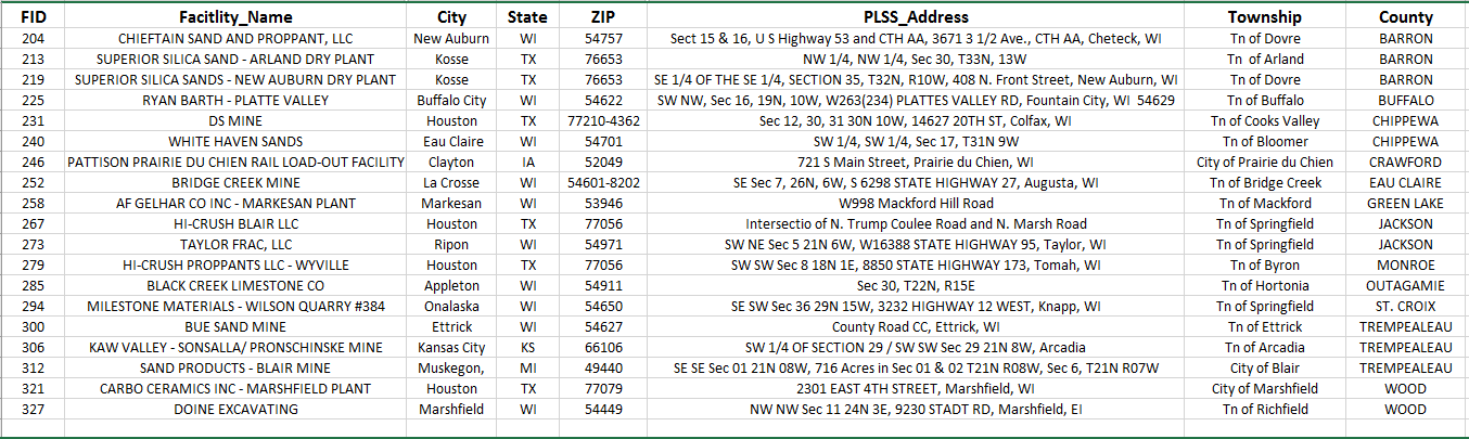
Part One of this exercise uses Pyscripter to perform a series of queries with attributes in the 'mines' feature class and ultimately create a new feature class accounting for all active mines lacking on-site rail loading stations and at a distance of at least 1.5 km from a rail line. These criteria are meant to indicate which mines must rely on trucks to transport the excavated frac sand mines' product. This segment of the project works to satisfy the first three of the five objectives. 

The first step required importing the arcpy module to the correct geodatabase and setting up the environments of the geodatabase to a readable and easily editable formula for the remaining length of the script. Variables were set for each of the following feature class layers in the geodatabase:

• "all_mines"
• "active_mines"
• "status_mines"
• "mines_norail"
• "wi"
• "rails_wtm"
• "mines_norail_final"

With the environments built, it was easy to arrange the necessary query statements which would reveal the target mines for the purposes of this project after running the script. The three statements can be seen in the text below, showing the final Python Script that was used to create the final mines feature class, used again in part two of the project. 

#-------------------------------------------------------------------------------

# Name:        Exercise 7 pt. 1

# Purpose:

# Author:      bauerkie

# Created:     10/04/2017

# Copyright:   (c) bauerkie 2017

# Licence:     <your licence>

#-------------------------------------------------------------------------------

import arcpy

from arcpy import env

arcpy.env.workspace ="Q:\StudentCoursework\CHupy\GEOG.337.001.2175\BAUERKIE\Labs\Exercises\ex7\ex7.gdb"

arcpy.env.overwriteOutput=True

#Set the Variables

all = "all_mines"

active = "active_mines"

Fc1 = "Site_Statu"

norail = "mines_norail"

wi = "wi"

rail = "rails_wtm"

worail = "mines_norail_final"

Fc2 = "Facility_T"

#Set up the field delimiters for the SQL statements

field1 = arcpy.AddFieldDelimiters(Fc1, "Site_Statu")

field2 = arcpy.AddFieldDelimiters(Fc2, "Facility_T")

#SQL statement to select active mines

activeSQLExp = field1 + " = " + "'Active'"

mineSQLExp = field2 + " LIKE " + "'%Mine%'"

norailSQL = "NOT" + field2 + " LIKE " + "'%Rail%'"

#Make a layer from the feature class with mine status = active

arcpy.MakeFeatureLayer_management (all, active, activeSQLExp)

#Make a layer from the feature class with facility type = mines

arcpy.MakeFeatureLayer_management(active, all, mineSQLExp)

#Make a layer from the feature class without rails

arcpy.MakeFeatureLayer_management(all, norail, norailSQL)

#SELECT

arcpy.SelectLayerByLocation_management(norail, "Intersect", wi)

arcpy.SelectLayerByLocation_management (norail, "WITHIN_A_DISTANCE", rail, "1.5 KILOMETER", "REMOVE_FROM_SELECTION")

arcpy.CopyFeatures_management(norail, worail)

print "The script is complete"

The successful execution of this script resulted in the creation of a new feature class hosting a total of 44 mines in its attribute table. 

Part Two:

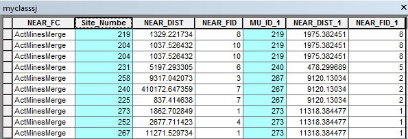
In Part Two, students use the closest facility solver on the network analysis toolbar to locate all the routes that trucks are likely to drive to get from each individual mine to the nearest rail transport. The resulting routes are then pieced out by separate county segments within each route. The "closest facility" solver is the best method for finding likely truck routes to rail terminals, in this case listing the rail terminals layer as the facilities, and the python-executed sand mine layer as the incidences. This will export routes in a stacked method, accounting for each of the trucks driving fragments of the same routes.  After solving, a total of  232 routes by county segments appeared most likely to host truck transportation of frac sands. An example of the attribute table is provided in Figure Two.

Figure Two: Attribute Table of Closest Facilities Route Analysis Solver

A series of analysis tools and table relationships outlined in ArcToolbox's Model Builder will reveal the estimated cost that this industry's transport has had on local roads and their upkeep by county, per year. The model used to determine each route's estimated costs is displayed next in Figure Three. This figure starts with the execution of the Network Analysis's Closest Facilities Solver explained previously and follows all the way through to the final calculation of a cost field for each route. The calculations used for calculating costs is explained further later on.

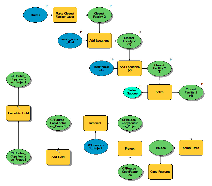
Figure Three: Arriving at Individual Route Costs

For the purposes of this assignment, an estimate of 50 round-trip truck excursions was used for each of the calculated mine site routes by county. The hypothetical road repair expense was priced at 2.2 cents per truck mile. Since the shape_length field is calculated in feet, the field values can each be divided by 5,280 feet to calculate miles, which was multiplied by 50 roundtrip trucks at a rate of $0.022 per mile. Figure Five shows the layer's attribute table after Model Builder has been run, and the new "Cost" field is generated using the following formula:

 "Cost" = "Shape_Length" / 5280 * 50 * 2 * 0.022

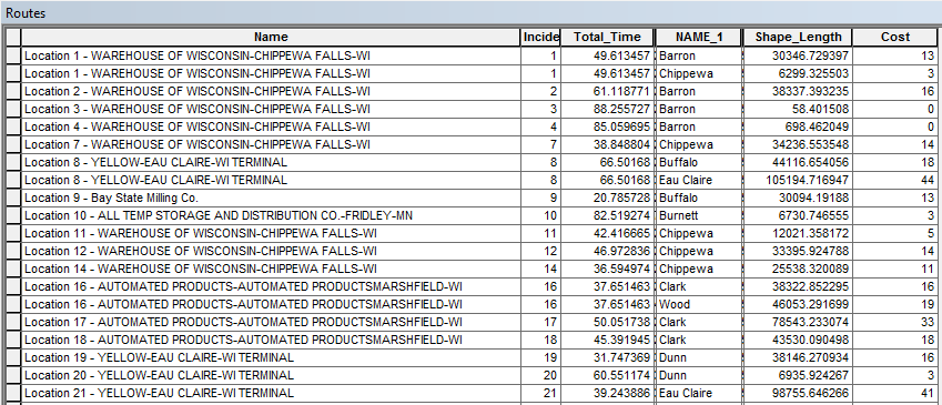
Figure Four: Routes Layer Attribute Table after Calculations from Model Builder

Finally, with the results of this additional, calculated "costs" field in the sand mine routes attribute table, the summary table of counties based on the sum of the costs of each route segment can be generated to reveal a table charting each mining county's total road repair costs per year. This table can be found in Figure Six of the next section: "Results." 

Results:

The results of each of the calculated sand mines and their corresponding calculated truck routes to the nearest rail terminal (outlined in parts one and two of the methods section) are displayed in the map labeled Figure Five below. The map reveals that most truck routes occur in clusters, indicating that many of the same roads are being utilized for transport, and likely, many of the same roads are taking the bulk of the county costs in damages. It also reveals that a large amount of mine sites are located in Trempeleau County, and many of them are using short road spans (likely to be local roads or highways) to get their product to their nearest road terminals.

Figure Five: Map showing calculated routes from each of the mine sites to their closest rail terminal

Figure Six is the resulting table after summarizing the cost field based on each of the counties hosting segments of the routes used from mine sites to terminals. It reveals that Chippewa County road segments take the largest cost burden at a rate of $610.00 per year as a result of sand mining industry traffic, while road segments in Wood County takes the least at only $2.00. Analyzing this chart can help to reveal which counties can afford to take additional road damages and which may consider diverting to the second next closest rail facilities to alleviate these areas of their road cost burdens.

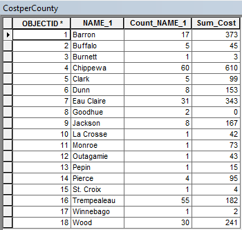
Figure Six: Table Totaling the Cost of Mine Transport Road Damages per County

Conclusion:

The totaling repair cost estimates of roads in each county as a result of truck traffic from frac sand mining was derived in the processes described in this lab. These types of infrastructure impacts are important to consider in assessing the potential hazards that these industries may inflict on road conditions when taking a look at these areas and assessing their ability to take on more of this industry.

Sources:

The White Papers, accessed through:
 http://midamericafreight.org/wp-content/uploads/FracSandWhitePaperDRAFT.pdf

Post 4: Sand Mining Suitability Project: Data Normalization, Geocoding, and Error Assessment

Introduction:

This lab introduced students to the process of geocoding various locations in ArcGIS using both automated program processes and the process of manually assessing and placing geocoded points based on the PLSS addresses of approximately nineteen sand mine locations in Western Wisconsin. The lab works to accompany an ongoing class community project seeks to ultimately develop a suitability/ risk model for sand mining in Western Wisconsin, and more specifically, in Trempealeau county.

The assignment ultimately entailed five key objectives:

1. Obtaining and normalizing the data address table
2. Auto-geocoding the mines using the ArcGIS geocoding toolbar and geocoding services provided by ESRI
3. Adding the Public Land Survey System (PLSS) base data layers through the University's SQL server
4. Manually locating/re-locating mines using the PLSS system description and previously added PLSS base data layers
5. Comparing the location results to actual placement data and the overall class collective 

Methods:

Figure 1: Original Excel Data

In beginning the lab, students were provided with a listed series of mines and their location information in an organized Excel file. The working list was divided up among students so that each mine site would be geocoded by approximately four students, and each student was designated approximately nineteen sand mine site locations for geocoding. Objective One required each student to pull their assigned mines and the data associated with each from the overall class data table (shown in Figure 1) and normalize the addresses into a separate Excel sheet file (Figure 2). Normalizing the data required the various types of addresses and their provided components to be pieced out from the facility address field into separate, individual fields, resulting in a separate field for each of the following: PLSS location or Street Address, city, town, county, state, and zip code.

A snapshot from the resulting normalized Excel table is pictured in Figure 2 below:

Figure 2: Normalized Excel Data for Mine Sites 

With the data now normalized, students were able to proceed to Objective Two, uploading the resulting sheet into ArcMap and logging in to ESRI's Enterprise server to enable the geocoding toolbar and begin locating each of the mine sites designated. ESRI's geocoding toolbar allows the geocoding process to be automated. The Address Inspector function located on the geocoding toolbar allows for the mine point placement, placement candidates, and the properties which were used in establishing the placement to be reviewed. After the original auto-placement of these mine sites, ArcMap generates an error table, which calculates the percent of accuracy and certainty in the mine site placement locations. The auto-placement error can be seen in Table 1.

Table 1: ArcMap Auto-Geocoding Error

While in most instances the auto-locator provided by ESRI does an adequate job in geocoding the locations of inputted address sites, the process is not always exact. For example, for addresses which possess ONLY a PLSS location description (in place of an actual street address), the automated geocoded location of these mines will not be accurately placed; instead, the mine's data point will fall in the center of it's associated town or city, and must be moved to the correct location from there. This can be accomplished through the various steps denoted in Objective Three and Four outlined below.

Figure 3: WiDNR2014 Database Layers Added to the Map

In phase four of the five part project, students were required to manually locate each of the remaining, unmatched mine sites using the PLSS address description and various PLSS feature class layers. Accessing these layers required the completion of the exercise's third objective: connecting with the University of Eau Claire: Geography Department's SQL Server and locating the necessary PLSS layers within the WiDNR2014 database. Once the connection was made, the layers shown in Figure 3 were able to be added to the map as base data, and symbolized so that each layer was decipherable with a distinctive colored outline and a hollowed center, so that the imagery basemap remained visible. From there, numeric labels were added to each of the layers to help guide the placement of the manually determined and  geocoded mine sites using the PLSS section, township, and quarter labels in each of the mine site addresses. Once the correct location of the sand mine was found, the "Pick Address from Map" button established the point's corrected location. The Match_Type field in the attribute table accounts for this alteration by replacing the original designated value 'A' (automated) to an 'M' (manual), signifying the change has been made. The process required all mine data point locations to be checked, and corrected where needed.

Lastly, Objective Five allowed students to compare their manual geocoding results with both the results of their peers as well as with the actual PLSS locations of the mines, while simultaneously assessing the degree of error that exists between each site placement. This task required students to merge their collected data with the class data AND the actual site location data before querying out their assigned mine IDs from the collective layer. This provided students with data for all geocoded placements for their 19 prescribed mines, their correct locations, and alternative geocoded site placements made by peers for the same mines. With this data now at hand, assessments about error can be made between each of the established placements per mine ID. Not surprisingly, each student's geocoded placements varied from the actual mine site location, at differing degrees. In order to measure the how drastic these distance differences were, a distance field needed to be added to a merged mines attribute table.

To establish this distance field, a total of three layers were pulled from the merged and queried layer representing the 19 mine IDs; these three new layers included "MyMines," "ClassMines," and "ActualMines." The "Near" tool was used twice to compare "MyMines" with "ActualMines" and "ClassMines" with "ActualMines." These results were then re-merged to reveal the distances between each geocoded mine and the actual mine site. A sample of the resulting table reporting distance error is pictured in Table 2. The first set of data refers to the self-geocoded distances results while the second set of data offers the geocoded distances of other students from the actual mine site locations.

Table 2: Geocoded Mine Sites Distance from Actual Mines Sites

Results:

The final result of the 19 geocoded mines which were manually located and placed, as previously described in objective four of the methods section, is pictured in Map 1 below. The map reveals how the PLSS system was used to narrow-in on each individual mine site location. A sample of the labeled grid system is showcased in the lower left corner of the map. Each mine was located using the numbers indicating township, section, and quarter section in the mine PLSS address.

In the PLSS system, Townships are established as a square block encompassing 36 square miles. These 36 square miles are then split into 36 individual square mile fragments that account for the 36 Sections. Each section, then, can be split further into four quarter sections. Directional values in the PLSS address indicate which of the section's four quadrants the mine in question is located in. 

Map 1: Geocoding Wisconsin Sand Mines with PLSS

The final placement of geocoded mine sites appear to be mostly in the western half and northcentral fragment of the state of Wisconsin, many clustered near the La Crosse and Eau Claire areas. The placement of these each of these mine sites can be compared to the correlating mine results of the class and the actual location of each mine in Map 2. 

Map 2: Wisconsin Sand Mines: Geocoding Error Sample Map

Map 2 makes an attempt to visually produce the distance error was calculated in Table 2

 of the methods section. It reveals the geocoding distances between a sample of manually self-plotted mines, some classmates same manually plotted mines, and the actual location of the mine. Hollowed stars mark the actual location of the sampled sand mines while varying colored circles represent the collective self- and peer- geocoded locations. The color of each point reveals how closely the plotted points were to the actual mine site locations. Green points symbolize close proximity to the actual location of the mine (between 480 and 1.300 feet), while red points symbolize the greatest amount of plotted distance error (12,000+ feet from the actual mine site location). Each plotted location includes a label of the mine's ID to match the geocoded locations with the actual locations accordingly. Pink text for the mine ID indicates a classmate's plotted geocode, while blue mine ID text showcases the self-attempts. Some of the clustered areas have been blown up and re-scaled for a more detailed distribution of the mine sites.

In analyzing the overall spatial distribution of the plotted mine sights, it seems that most of the plotted mine sites generally lie in near proximity to the mine site's actual location (within a mile of the target site, or symbolized by the first three distance ranges in the map's legend). As evident within the map's data, there was not always a classmate attempt to compare to for each of the mine sites produced. In this sampled section, only four of their contributions are made apparent for comparison. Some outliers in the data include mine ID 240, whose red color symbolizes a large distance error from the actual mine site, which can be located approximately 410,000 feet north of the attempted plotted site. This error was likely made due to misreading the PLSS address details. A second error is evident with the actual plotted site 213, for which there are no corresponding geocoded attempts, neither self-made or peer-produced. This error was also likely due to human error in piecing out a sample of the 19 mine site IDs to showcase for the error map. 

Discussion:

The readings on Lo's "Data Quality and Data Standards" discusses the difference between accuracy and precision in a geographic context. Accuracy is a measure of how closely the data and attributes between the representation and the real world resemble one another. Precision, on the other hand, makes a determination of how exact the location measurement of the representative data resembles to the location of the actual data as it exists in the real world. Many of the mines situated in clusters near to one another show an example of precision error. Mines in these instances are placed in near proximity to one another, but it would be nearly impossible to pin-point the exact placement of the points determining the actual mine. An example of accuracy error can be seen with the plotted mines distanced far from one another. Mines such as Mine Site 240 show two separate locations which in no way should resemble one another. Of the three error types: gross, systemic and random, that which is most apparent here are likely to be gross error, or errors which could be avoided with a few more random checks of the plotted data.

Conclusion:

This lab offered students the opportunity to familiarize themselves with two different types of geocoding and the potential errors that can arise from its use. Having an awareness of these potential errors will prove useful in future geocoding activities which may arise in later projects so that these errors can hopefully be avoided. The exercise was also a good activity for reviewing the PLSS system and learning how to navigate the overall grid system to find various mine site locations. Further analysis on each of these mine sites will be made in future blogs to come in completing the Trempealeau County Sand Mine class project through additional class organized exercises.